Combine ChIP-seq peaks from multiple replicates via consensus voting
Published on
As in most of biology, having biological replicates in ChIP-seq experiments is important to ensure external validity.
Or, in simpler words, your low-q-value peak from a single sample only means that the peak was definitely there in this one sample. Without replicates, you don’t know if this peak is reliably there across samples or was specific to that one sample at that one time.
So, in order to know that your results are reliable and can be expected to replicate in other similar experiments, you should replicate them yourself on different biological samples. The more diverse your replicates, the more externally valid your findings. For instance, if all your replicates come from the same inbred strain, you can conclude that your findings probably generalize to most individuals in that strain but may be caused by the strain’s genotype and not generalize to the whole population.
But say you do have biological replicates — how do you analyze them? While tools for differential analysis of peaks typically know how to deal with replicates, tools for peak calling (such as MACS) deal only with a single replicate at a time. This is a problem if you are only interested in finding transcription factor binding sites.
Often people seem to resort to either intersecting or taking the union of all peaks just because it’s very easy to do using bedtools. However, as Yang et al. argue, doing so will result in high false negative and false positive rates, respectively. Instead, they propose a compromise: call a consensus peak if it’s supported by at least a certain number of replicates — say, by at least half of them. But unlike simple union or intersection, there do not appear to be any ready-to-use tools to perform this kind of analysis.
So here I’ll explain how to use R/Bioconductor to find regions that are covered by at least a given number of replicate peaks. Note that my approach does not correspond directly to any of the 4 approaches described by Yang et al. Their method results in a smaller number of wider peaks, but parts of those consensus peaks may have smaller coverage as shown below.
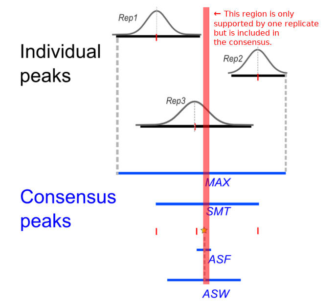
This could be a problem when peaks spanning hundreds or thousands of bp overlap only a little. A better approach would be to first to identify regions supported by the given number of replicates and then optionally merge those that are close to each other, which I’ll also show how to do.
Of course this is very subjective and arbitrary, and ideally we would use a robust statistical model instead of a hand-picked threshold. And there are some tools that attempt this:
I discussed GenoGAM with its authors last year, but I am yet to study and compare the other ones.
Calling consensus peaks in Bioconductor
First, load the Bioconductor libraries to work with genomic ranges:
library(rtracklayer)
library(GenomicRanges)
Get the list of .narrowPeak files in the current
directory. We’ll treat them all as replicates. The same code should work
with .bed or .gff files.
peak_files <- list.files(pattern = ".*\\.narrowPeak")
peak_files
## [1] "NRF2SFN-Chorley-rep1_bw300_narrow_peaks.narrowPeak"
## [2] "NRF2SFN-Chorley-rep2_bw300_narrow_peaks.narrowPeak"
## [3] "NRF2SFN-Chorley-rep3_bw300_narrow_peaks.narrowPeak"Read these files using rtracklayer’s import
function:
peak_granges <- lapply(peak_files, import)
peak_granges
## [[1]]
## GRanges object with 1415 ranges and 6 metadata columns:
## seqnames ranges strand | name
## <Rle> <IRanges> <Rle> | <character>
## [1] NC_000001.11 10041-10186 * | NRF2SFN-Chorley-rep1_bw300_narrow_peak_1
## [2] NC_000001.11 629597-629707 * | NRF2SFN-Chorley-rep1_bw300_narrow_peak_2
## [3] NC_000001.11 630278-630444 * | NRF2SFN-Chorley-rep1_bw300_narrow_peak_3
## [4] NC_000001.11 631154-631304 * | NRF2SFN-Chorley-rep1_bw300_narrow_peak_4
## [5] NC_000001.11 631961-632210 * | NRF2SFN-Chorley-rep1_bw300_narrow_peak_5
## ... ... ... ... . ...
## [1411] NW_017852933.1 1174567-1174677 * | NRF2SFN-Chorley-rep1_bw300_narrow_peak_1411
## [1412] NW_017852933.1 1593093-1593226 * | NRF2SFN-Chorley-rep1_bw300_narrow_peak_1412
## [1413] NW_018654708.1 221820-221930 * | NRF2SFN-Chorley-rep1_bw300_narrow_peak_1413
## [1414] NW_018654713.1 29933-30043 * | NRF2SFN-Chorley-rep1_bw300_narrow_peak_1414
## [1415] NW_019805500.1 69753-69895 * | NRF2SFN-Chorley-rep1_bw300_narrow_peak_1415
## score signalValue pValue qValue peak
## <numeric> <numeric> <numeric> <numeric> <integer>
## [1] 27 5.17033 6.91041 2.79078 38
## [2] 66 3.80497 11.22005 6.63982 82
## [3] 93 4.31874 14.1121 9.31245 98
## [4] 50 3.50501 9.46955 5.06445 99
## [5] 77 4.25812 12.40796 7.76729 174
## ... ... ... ... ... ...
## [1411] 31 4.58205 7.31183 3.15002 63
## [1412] 158 10.99692 21.19611 15.89375 50
## [1413] 60 5.71026 10.64406 6.09574 23
## [1414] 53 6.15752 9.80128 5.37605 17
## [1415] 47 5.49846 9.13087 4.7435 78
## -------
## seqinfo: 81 sequences from an unspecified genome; no seqlengths
##
## [[2]]
## GRanges object with 10073 ranges and 6 metadata columns:
## seqnames ranges strand | name
## <Rle> <IRanges> <Rle> | <character>
## [1] NC_000001.11 9913-10101 * | NRF2SFN-Chorley-rep2_bw300_narrow_peak_1
## [2] NC_000001.11 118531-118688 * | NRF2SFN-Chorley-rep2_bw300_narrow_peak_2
## [3] NC_000001.11 175750-175907 * | NRF2SFN-Chorley-rep2_bw300_narrow_peak_3
## [4] NC_000001.11 180786-181117 * | NRF2SFN-Chorley-rep2_bw300_narrow_peak_4
## [5] NC_000001.11 295097-295254 * | NRF2SFN-Chorley-rep2_bw300_narrow_peak_5
## ... ... ... ... . ...
## [10069] NW_019805499.1 41689-41864 * | NRF2SFN-Chorley-rep2_bw300_narrow_peak_10069
## [10070] NW_019805499.1 42535-42692 * | NRF2SFN-Chorley-rep2_bw300_narrow_peak_10070
## [10071] NW_019805500.1 15499-15656 * | NRF2SFN-Chorley-rep2_bw300_narrow_peak_10071
## [10072] NW_019805501.1 42374-42531 * | NRF2SFN-Chorley-rep2_bw300_narrow_peak_10072
## [10073] NW_019805503.1 32183-32340 * | NRF2SFN-Chorley-rep2_bw300_narrow_peak_10073
## score signalValue pValue qValue peak
## <numeric> <numeric> <numeric> <numeric> <integer>
## [1] 56 6.82969 10.16471 5.62669 138
## [2] 30 3.84819 7.00974 3.01917 96
## [3] 15 2.8959 5.1229 1.53902 65
## [4] 64 7.20184 11.08078 6.47703 95
## [5] 25 3.75744 6.16293 2.50373 104
## ... ... ... ... ... ...
## [10069] 67 5.79181 11.53681 6.76819 34
## [10070] 30 3.8263 6.76788 3.00398 61
## [10071] 24 3.74499 6.07139 2.41671 109
## [10072] 30 3.8263 6.76788 3.00398 115
## [10073] 30 3.86121 7.17009 3.01917 23
## -------
## seqinfo: 250 sequences from an unspecified genome; no seqlengths
##
## [[3]]
## GRanges object with 5834 ranges and 6 metadata columns:
## seqnames ranges strand | name
## <Rle> <IRanges> <Rle> | <character>
## [1] NC_000001.11 75561-75825 * | NRF2SFN-Chorley-rep3_bw300_narrow_peak_1
## [2] NC_000001.11 118452-118776 * | NRF2SFN-Chorley-rep3_bw300_narrow_peak_2
## [3] NC_000001.11 295059-295342 * | NRF2SFN-Chorley-rep3_bw300_narrow_peak_3
## [4] NC_000001.11 376867-377338 * | NRF2SFN-Chorley-rep3_bw300_narrow_peak_4
## [5] NC_000001.11 474500-474783 * | NRF2SFN-Chorley-rep3_bw300_narrow_peak_5
## ... ... ... ... . ...
## [5830] NW_019805495.1 242418-242709 * | NRF2SFN-Chorley-rep3_bw300_narrow_peak_5830
## [5831] NW_019805495.1 258219-258668 * | NRF2SFN-Chorley-rep3_bw300_narrow_peak_5831
## [5832] NW_019805496.1 127568-127832 * | NRF2SFN-Chorley-rep3_bw300_narrow_peak_5832
## [5833] NW_019805499.1 30032-30296 * | NRF2SFN-Chorley-rep3_bw300_narrow_peak_5833
## [5834] NW_019805500.1 7260-7524 * | NRF2SFN-Chorley-rep3_bw300_narrow_peak_5834
## score signalValue pValue qValue peak
## <numeric> <numeric> <numeric> <numeric> <integer>
## [1] 30 4.46341 6.72273 3.00157 88
## [2] 76 7.14145 12.01206 7.62227 66
## [3] 57 6.52364 9.85515 5.70239 27
## [4] 225 14.2829 28.09008 22.54761 253
## [5] 55 6.4522 9.65794 5.5344 181
## ... ... ... ... ... ...
## [5830] 21 4.07727 5.38735 2.108 182
## [5831] 42 5.28269 8.11069 4.24385 249
## [5832] 43 5.35609 8.42216 4.39757 73
## [5833] 42 5.28269 8.11069 4.24385 104
## [5834] 30 4.46341 6.72273 3.00157 180
## -------
## seqinfo: 170 sequences from an unspecified genome; no seqlengthspeak_ranges is a simple R list with 3 elements, which
individually are GRanges objects. Now let’s turn this list
into a GRangesList, which in this case is more convenient
to work with.
peak_grangeslist <- GRangesList(peak_granges)
peak_grangeslist
## GRangesList object of length 3:
## [[1]]
## GRanges object with 1415 ranges and 6 metadata columns:
## seqnames ranges strand | name
## <Rle> <IRanges> <Rle> | <character>
## [1] NC_000001.11 10041-10186 * | NRF2SFN-Chorley-rep1_bw300_narrow_peak_1
## [2] NC_000001.11 629597-629707 * | NRF2SFN-Chorley-rep1_bw300_narrow_peak_2
## [3] NC_000001.11 630278-630444 * | NRF2SFN-Chorley-rep1_bw300_narrow_peak_3
## [4] NC_000001.11 631154-631304 * | NRF2SFN-Chorley-rep1_bw300_narrow_peak_4
## [5] NC_000001.11 631961-632210 * | NRF2SFN-Chorley-rep1_bw300_narrow_peak_5
## ... ... ... ... . ...
## [1411] NW_017852933.1 1174567-1174677 * | NRF2SFN-Chorley-rep1_bw300_narrow_peak_1411
## [1412] NW_017852933.1 1593093-1593226 * | NRF2SFN-Chorley-rep1_bw300_narrow_peak_1412
## [1413] NW_018654708.1 221820-221930 * | NRF2SFN-Chorley-rep1_bw300_narrow_peak_1413
## [1414] NW_018654713.1 29933-30043 * | NRF2SFN-Chorley-rep1_bw300_narrow_peak_1414
## [1415] NW_019805500.1 69753-69895 * | NRF2SFN-Chorley-rep1_bw300_narrow_peak_1415
## score signalValue pValue qValue peak
## <numeric> <numeric> <numeric> <numeric> <integer>
## [1] 27 5.17033 6.91041 2.79078 38
## [2] 66 3.80497 11.22005 6.63982 82
## [3] 93 4.31874 14.1121 9.31245 98
## [4] 50 3.50501 9.46955 5.06445 99
## [5] 77 4.25812 12.40796 7.76729 174
## ... ... ... ... ... ...
## [1411] 31 4.58205 7.31183 3.15002 63
## [1412] 158 10.99692 21.19611 15.89375 50
## [1413] 60 5.71026 10.64406 6.09574 23
## [1414] 53 6.15752 9.80128 5.37605 17
## [1415] 47 5.49846 9.13087 4.7435 78
##
## ...
## <2 more elements>
## -------
## seqinfo: 299 sequences from an unspecified genome; no seqlengthsNow, find the genome regions which are covered by at least 2 of the 3 sets of peaks:
peak_coverage <- coverage(peak_grangeslist)
peak_coverage
## RleList of length 299
## $NC_000001.11
## integer-Rle of length 248946484 with 3023 runs
## Lengths: 9912 128 61 85 65374 265 ... 220661 275 137 85 197 84
## Values : 0 1 2 1 0 1 ... 0 1 2 1 2 1
##
## $NC_000002.12
## integer-Rle of length 242183602 with 1773 runs
## Lengths: 214478 265 588943 158 260 ... 288 50217 103 159 28
## Values : 0 1 0 1 0 ... 1 0 1 2 1
##
## $NC_000003.12
## integer-Rle of length 198174065 with 1492 runs
## Lengths: 9884 259 73 209 217 ... 158 98693 221 4926 294
## Values : 0 1 2 3 2 ... 1 0 1 0 1
##
## $NC_000004.12
## integer-Rle of length 190204610 with 1998 runs
## Lengths: 9848 94 53 243 44 62 ... 1005 11 162 106 23142 170
## Values : 0 1 2 3 2 1 ... 0 1 2 1 0 1
##
## $NC_000005.10
## integer-Rle of length 181450116 with 1874 runs
## Lengths: 9901 7 97 1388 54 ... 112 158 202 6807 1286
## Values : 0 1 2 3 2 ... 1 2 1 0 1
##
## ...
## <294 more elements>peak_coverage is a list of numbers for every single
genome position, encoded into an efficient structure Rle. Now, using the
slice function, let’s get the regions in the genome where
coverage is at least 2:
covered_ranges <- slice(peak_coverage, lower=2, rangesOnly=T)
covered_ranges
## IRangesList of length 299
## $NC_000001.11
## IRanges object with 154 ranges and 0 metadata columns:
## start end width
## <integer> <integer> <integer>
## [1] 10041 10101 61
## [2] 118531 118688 158
## [3] 295097 295254 158
## [4] 377069 377226 158
## [5] 709516 709673 158
## ... ... ... ...
## [150] 228636089 228636238 150
## [151] 243037096 243037253 158
## [152] 244523624 244523802 179
## [153] 248945982 248946118 137
## [154] 248946204 248946400 197
##
## ...
## <298 more elements>This is a simple IRangesList object; let’s covert it to
a GRanges object:
covered_granges <- GRanges(covered_ranges)
covered_granges
## GRanges object with 1401 ranges and 0 metadata columns:
## seqnames ranges strand
## <Rle> <IRanges> <Rle>
## [1] NC_000001.11 10041-10101 *
## [2] NC_000001.11 118531-118688 *
## [3] NC_000001.11 295097-295254 *
## [4] NC_000001.11 377069-377226 *
## [5] NC_000001.11 709516-709673 *
## ... ... ... ...
## [1397] NT_187617.1 59572-59732 *
## [1398] NW_003315930.1 14229-14368 *
## [1399] NW_003315952.3 57671-57785 *
## [1400] NW_003315959.1 134807-134820 *
## [1401] NW_003571050.1 380055-380202 *
## -------
## seqinfo: 299 sequences from an unspecified genome; no seqlengthsAnd we are done! We can also save these regions as a
.bed file using rtracklayer’s export:
export(covered_granges, "consensus.bed")Merging nearby peaks
As I mentioned at the beginning, you might want to merge the peaks
that are close to each other to avoid having many small fragments. In
Bioconductor, you can do that using the min.gapwidth
parameters to reduce. For example, this will merge the
peaks that are separated by no more than 30 bp:
reduce(covered_granges, min.gapwidth=31)## GRanges object with 1379 ranges and 0 metadata columns:
## seqnames ranges strand
## <Rle> <IRanges> <Rle>
## [1] NC_000001.11 10041-10101 *
## [2] NC_000001.11 118531-118688 *
## [3] NC_000001.11 295097-295254 *
## [4] NC_000001.11 377069-377226 *
## [5] NC_000001.11 709516-709673 *
## ... ... ... ...
## [1375] NT_187617.1 59572-59732 *
## [1376] NW_003315930.1 14229-14368 *
## [1377] NW_003315952.3 57671-57785 *
## [1378] NW_003315959.1 134807-134820 *
## [1379] NW_003571050.1 380055-380202 *
## -------
## seqinfo: 299 sequences from an unspecified genome; no seqlengthsAs you can see, this reduced the number of ranges from 1401 to 1379.