Theory behind RSEM
Published on
In this article, I will walk through and try to explain a 2009 paper RNA-Seq gene expression estimation with read mapping uncertainty by Bo Li, Victor Ruotti, Ron M. Stewart, James A. Thomson, and Colin N. Dewey.
I will also occasionally refer to a 2011 paper by Bo Li and Colin N. Dewey, RSEM: accurate transcript quantification from RNA-Seq data with or without a reference genome.
Together, the two papers explain the theory behind the software package for estimating gene and isoform expression levels RSEM.
Motivation
An RNA-Seq experiment proceeds roughly as follows:
- A class of RNA molecules (e.g., mRNA) is extracted from a biological sample.
- The molecules are fragmented. The size of RNA fragments is in the hundreds of nucleotides.
- A random sample of the RNA fragments is sequenced. The obtained sequences are called reads and usually have a fixed length from 50 to 250 nucleotides.
Typically (but not always), the RNA is reverse-transcribed to DNA either before or after fragmentation, and it is the DNA that gets sequenced, but that’s irrelevant for us here.
The goal of the RNA-Seq data analysis is, given the reads and a list of known gene isoforms (all possible RNA sequences), estimate the relative number of RNA molecules (transcripts) of each isoform in the original biological sample.
So, for instance, given two isoforms
(isoform 1) AAAAAAAAAAA
(isoform 2) UUUUUUUUUUU
and three reads
(read 1)    AAAAAAA
(read 2)    UUUUUUU
(read 3)    AAAAAAA
we might estimate that rougly \(2/3\) of all transcripts in the biological sample were from isoform 1 and \(1/3\) were from isoform 2.
A simple estimation method is to count the reads that align to each isoform and then adjust the counts for the number of reads and isoform sizes.
However, not all reads align to a single isoform. Isoforms of the same gene are highly similar: they all are built from the same small set of segments (exons). Different genes may also be highly similar. More than a half of the reads in any given experiment may map to more than one isoform. Such reads are called multireads.
We could just ignore multireads and consider only the reads that unambiguously map to one isoform. One problem with this is discarding a lot of useful data. But more importantly, without a careful adjustment, discarding multireads introduces a bias: we will underestimate the abundance of genes that have many active isoforms or other similar genes, as these genes are more likely to produce multireads.
The paper describes a probabilistic model and a computational method to estimate isoform abundances based on all available reads, including multireads.
Simplifications
As in the original paper, we will assume single-end reads and ignore quality scores. Besides, we will make two addional assumptions compared to the paper:
- The protocol is strand-specific; that is, we will assume the orientation of the reads is known just so that we have fewer variables to model.
- All reads come from a known list of isoforms. Therefore, we will not consider the “noise” isoform (\(i=0\) in the paper).
Notation and variables
\(N\) is the total number of reads (called library size); \(n=1,\ldots,N\).
\(M\) is the number of known isoforms; \(i=1,\ldots,M\).
\(L\) is the read length.
\(l_i\) is the length of isoform \(i\); \(j=1,\ldots,l_i\).
\(R_n\) is the sequence of read \(n\).
Read \(n\) is assumed to start at a position \(S_n\in[1,l_i]\) in the isoform \(G_n=i\in[1,M]\).
\(\tau_i\) is the fraction of transcripts that belong to isoform \(i\) out of all transcripts in the sample. When multiplied by million, it is the transcripts per million (TPM) measure.
\(\theta_i\) is the prior probability that any single read is derived from isoform \(i\): \(\theta_i=p(G_n=i)\). Because longer isoforms are expected to produce proportionally more fragments and reads, the relationship between \(\tau_i\) and \(\theta_i\) is: \[\theta_i=\frac{\tau_i\cdot l_i}{\sum_{k=1}^{M}\tau_{k}\cdot l_{k}},\] \[\tau_i=\frac{\theta_i/l_i}{\sum_{k=1}^{M}\theta_{k}/l_{k}}.\]
In other words, \(\theta_i\propto \tau_i\cdot l_i\) subject to \(\sum_i \theta_i = \sum_i \tau_i = 1\).
The symbol \(\propto\) used above means “proportional to”. The formula \(\theta_i\propto \tau_i\cdot l_i\) means that \(\theta_i/(\tau_i\cdot l_i)\) is constant and does not depend on \(i\). Similarly, \(p(\theta)\propto 1\) means that \(\theta\) has a constant (uniform) probability density.
Vectors of parameters are denoted by letters without indices:
- \(R=(R_1, \ldots, R_N)\)
- \(G=(G_1, \ldots, G_N)\)
- \(S=(S_1, \ldots, S_N)\)
- \(\tau=(\tau_1, \ldots, \tau_M)\)
- \(\theta=(\theta_1, \ldots, \theta_M)\)
\(\mathbb{I}\) is the indicator function: \(\mathbb{I}_p\) is equal to \(1\) if \(p\) is true and \(0\) otherwise.
Thus, we have five vector-valued random variables (of different dimensions!): \(\theta, \tau, G, S, R\). Of these, \(R\) is the observed data, and \(\theta\) and \(\tau\) are the unknown parameters that we wish to estimate from the data. \(G\) and \(S\) are unobserved variables that we are not directly interested in, but they are necessary to build the model.
Vectors \(\tau\) and \(\theta\) are equivalent in the sense that they carry the same information, just on different scales. Once we estimate \(\theta\), we can get an equivalent estimate of \(\tau\), and vice versa, using the conversion formulae given above.
We call \(\theta\) a random variable in the Bayesian sense. It is random because its value is not known and some values of \(\theta\) are more consistent with the data than the others. There is no particular random process that generates \(\theta\), so it is not random in the classical (frequentist) sense.
Probabilistic approach
What does an estimate of \(\theta\) (or \(\tau\), which is usually more interesting) look like? The most general form is the full posterior probability distribution \(p(\tau|R)\). In practice, we need to summarize the distribution to make sense of it. Some useful summaries are:
- The maximum a posteriori (MAP) value, or the mode of the posterior distribution, is the value of \(\tau\) for which \(p(\tau|R)\) has the greatest possible value. This is, roughly speaking, the most likely value of \(\tau\) under our model given the observed data.
- An uncertainty interval \((\tau^1, \tau^2)\) at level \(\gamma\) gives a plausible range of values that \(\tau\) might take: \[p(\tau^1 < \tau < \tau^2|R)=\gamma.\]
- If we are interested in one or a handful of genes or isoforms, we may want to plot the marginal distributions \(p(\tau_i|R)\).
- If we are interested in the differential expression of isoforms \(i\) and \(k\) within the same experiment, we can compute \[p(\tau_i > \tau_k|R).\] Or, we can compare expression in two independent experiments \((\tau, R)\) and \((\tau',R')\) by computing \[p(\tau_i > \tau_i'|R,R').\]
Generative model
We begin by formulating a generative model, a probabilistic process that conceptually generates our data.
Li et al. suggest a model where \(G_n\), \(S_n\), and \(R_n\) are generated for every \(n\) as follows:
Draw \(G_n\) from the set \(\{1,\ldots,M\}\) of all isoforms according to the probabilities \(\theta\): \[p(G_n=i|\theta)=\theta_i.\]
Choose where on the isoform the read will start according to the read start position distribution (RSPD) \(p(S_n|G_n)\).
The authors suggest two uniform distributions: for poly(A)+ RNA \[p(S_n=j|G_n=i)=\frac{1}{l_i} \cdot \mathbb{I}_{1\leq j\leq l_i}\] and for poly(A)- RNA \[p(S_n=j|G_n=i)=\frac{1}{l_i-L+1} \cdot \mathbb{I}_{1\leq j\leq (l_i-L+1)}.\]
The exact form of the RSPD doesn’t matter as long as it is known in advance. The paper also shows how to estimate the RSPD from data; we will not cover that here.
The read \(R_n\) is generated by sequencing the isoform \(G_n\) starting from the position \(S_n\). If sequencing was perfect, this would be deterministic: \(R_n\) would contain exactly the bases \(S_n, S_n+1, \ldots, S_n+L-1\) from \(G_n\). In reality, sequencing errors happen, and we can read a slightly different sequence. Hence \(R_n\) is also a random variable with some conditional distribution \(p(R_n|G_n,S_n)\).
As with RSPD, we don’t care about the particular form of the conditional probability \(p(R_n|G_n,S_n)\). In the simplest case, it would assign a fixed probability such as \(10^{-3}\) to each mismatch between the read and the isoform. More realistically, the error probability would increase towards the end of the read. Better yet, we could extend the model to take quality scores into account.
Note that this model does not accurately represent the physics of an RNA-Seq experiment. In particular, it does not model fragmentation. Essentially, the model assumes that the fragment size is constant and equal to the read length. This is addressed in the 2011 paper, although the model there is still backwards: they first pick an isoform and then a fragment from it, whereas in reality we pick a fragment at random from a common pool, and that determines the isoform. This is the reason why \(\theta\) does not represent the isoform frequencies and has to be further normalized by the isoform lengths to obtain \(\tau\).
A generative model does not have to match exactly the true data generation process as long as the joint distribution \(p(G,S,R|\theta)\) fits the reality. Here, the authors saw a way to simplify a model without sacrificing its adequacy much.
This model describes the following Bayesian network:

We can write the joint probability as \[p(G,S,R|\theta)=\prod_{n=1}^N p(G_n,S_n,R_n|\theta)=\prod_{n=1}^N p(G_n|\theta)p(S_n|G_n)p(R_n|G_n,S_n)\label{JOINT}\tag{JOINT}.\]
Finding \(\theta\)
How do we get from \(p(G,S,R|\theta)\) to \(p(\theta|R)\)?
We start by marginalizing out the unknowns \(G_n\) and \(S_n\):
\[\begin{align*} p(R|\theta)=\prod_{n=1}^N p(R_n|\theta) & = \prod_{n=1}^N\sum_{i=1}^M\sum_{j=1}^{l_i} p(R_n,G_n=i,S_n=j|\theta) \\ &=\prod_{n=1}^N\sum_{i=1}^M\sum_{j=1}^{l_i} p(R_n|G_n=i,S_n=j) p(S_n|G_n) \theta_i . \end{align*}\]
Then apply Bayes’ theorem to find \(\theta\):
\[p(\theta|R)=\frac{p(R|\theta)p(\theta)}{p(R)}.\]
We could expand \(p(R)\) as \(\int p(R|\theta)p(\theta)d\theta\), but since \(p(R)\) does not depend on \(\theta\), we won’t need to calculate it.
Choosing the prior
\(p(\theta)\) is the prior probability density of \(\theta\). Let’s pretend that we do not have any prior information on the isoform expression levels. Then it may seem reasonable to assume a uniform prior probability density \(p(\theta)\propto 1\).
There is a subtle issue with this. Recall that the isoform expression levels are represented by the vector \(\tau\), not \(\theta\). The vector \(\theta\) is “inflated” by the isoform lengths to account for the effect that longer isoforms produce more reads.
Therefore, the prior \(p(\theta)\propto 1\) corresponds to the (unfounded) assumption that shorter isoforms are somehow a priori more expressed than longer ones.
A better prior for \(\theta\) might be the one for which the vector \[\tau(\theta)=(\tau_1(\theta),\ldots,\tau_M(\theta))=\left(\frac{\theta_1/l_1}{\sum_{k=1}^M \theta_k/l_k},\ldots,\frac{\theta_M/l_M}{\sum_{k=1}^M \theta_k/l_k}\right)\] is uniformly distributed on the unit simplex. The probability density of such distribution is
\[p(\theta)=(n-1)!\cdot\frac{\partial(\tau_1,\ldots,\tau_{M-1})}{\partial(\theta_1,\ldots,\theta_{M-1})},\]
where the “fraction” on the right is the Jacobian determinant. (We parameterize \(\theta\) and \(\tau\) distributions by the first \(M-1\) vector components, viewing \(\theta_M=1-\sum_{k=1}^{M-1}\theta_k\) and \(\tau_M=1-\sum_{k=1}^{M-1} \tau_k\) as functions.)
How much do the different priors affect the results? It is not clear. Li et al. use the uniform prior on \(\theta\) implicitly in the 2009 paper by computing the maximum likelihood estimate and explicitly in the 2011 paper, when computing credible intervals. In the latter paper, they note:
CIs estimated from data simulated with the mouse Ensembl annotation were less accurate (Additional file 7). We investigated why the CIs were less accurate on this set and found that many of the CIs were biased downward due to the Dirichlet prior and the larger number of transcripts in the Ensembl set.
I haven’t tested yet whether the uniform \(\tau\) prior improves these CIs.
In this article, we will follow the lead of Li et al. and assume \(p(\theta)\propto 1\).
EM explanation
The EM (“expectation-maximization”) algorithm is used to find the maximum a posteriori estimate of \(\theta\). As Li et al. point out, the EM algorithm can be viewed as repeated “rescuing” of multireads. Let’s see what that means.
In this section, we will assume that a read either maps to an isoform perfectly or does not map to it at all, and that it can map to each isoform only once (though it can map to several isoforms at the same time). This is just to simplify the presentation. The algorithm and its derivation, which are presented in the next section, can handle the general case.
Intuition
First, consider a case of only two expressed isoforms (\(M=2\)). In general, there will be some number of reads, say, \(N_1\), that map only to isoform 1, some other number, \(N_2\), of reads that map only to isoform 2. Finally, there will be \(N_{12}=N-N_1-N_2\) reads that map equally well to both isoforms.
The easiest way to estimate \(\theta\) is by considering only unambiguously mapped reads. This leads to the “zeroth” approximations
\[\begin{align*} \theta^{(0)}_1&=N_1/(N_1+N_2),\\ \theta^{(0)}_2&=N_2/(N_1+N_2). \end{align*}\]
This is the best we can do considering just \(N_1\) and \(N_2\). To improve our estimate, we need to extract some information from \(N_{12}\).
Consider a particular multiread \(n\). Can we guess to which isoform it belongs? No, it maps equally well to both. But can we guess how many of the multireads come from each isoform? The more expressed an isoform is, the more reads we expect it to contribute to \(N_{12}\). How do we know how much each isoform is expressed? We don’t — if we knew, we wouldn’t need the algorithm — but we can make a reasonable guess based on the estimate \(\theta^{(0)}\).
We need to be careful, though. Would it be valid to estimate the fraction of ambiguous reads that come from isoform 1 as \(\theta^{(0)}_1\)?
Suppose that isoform 1 is much shorter than isoform 2: \(l_1 \ll l_2\). Now consider any particular ambiguous read \(R_n\). Does the fact that \(l_1 \ll l_2\) increase the probability that this read comes from the longer isoform, i.e. that \(G_n=2\)?
No — because, according to our assumptions made earlier in this section, \(R_n\) maps to either isoform only once. The number of all fragments produced by isoform \(i\) is proportional to \(\theta_i\); but the number of fragments capable of producing a particular read, \(R_n\), is proportional to the transcript abundance, \(\tau_i\). The longer an isoform, the more fragments it will produce, but also the lower fraction of these fragments will look anything like \(R_n\).
Therefore, we partition the \(N_{12}\) ambiguous reads between the two isoforms in proportion \(\tau^{(0)}_1:\tau^{(0)}_2\), where \(\tau^{(0)}\) is derived from \(\theta^{(0)}\) according to the usual formula (see Notation and variables).
Partitioning the multireads gives us the updated counts: \(N_1 + N_{12}\cdot\tau^{(0)}_1\) for isoform 1 vs. \(N_2 + N_{12}\cdot\tau^{(0)}_2\) for isoform 2. These updated counts lead us to a new estimate of \(\theta\), \(\theta^{(1)}\): \[\theta^{(1)}_i = \frac{N_i+N_{12}\cdot\tau^{(0)}_i}{N}.\]
And the cycle repeats. We can repeat this procedure until we notice that \(\theta^{(r+1)}\) does not differ much from \(\theta^{(r)}\).
Simulation
For a higher number of isoforms, the computations are analogous. To see how this works out in practice, consider the following simulated example with 3 isoforms. You can download the R script performing the simulation.
The true values of \(l\) and \(\theta\) are:
\[ \begin{array}{c|rr} i & l_i & \theta_i \\ \hline 1 & 300 & 0.60 \\ 2 & 1000 & 0.10 \\ 3 & 2000 & 0.30 \\ \end{array} \]
The counts obtained from a thousand RNA-Seq reads are:
\[ \begin{array}{lll} N_1 = 111 & N_{12} = 69 & N_{123} = 144 \\ N_2 = 26 & N_{13} = 311 \\ N_3 = 186 & N_{23} = 153 \\ \end{array} \]
Amazingly, under the assumptions introduced in this section, we don’t need to know the actual reads and how they map to the isoforms — we only need the six numbers above.
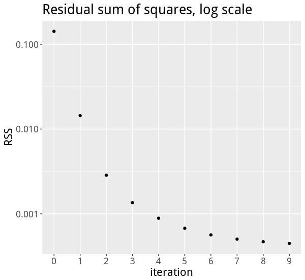
The first five successive approximations for \(\theta\) made by the EM algorithm are:
\[ \begin{array}{r|rrrrr} i & \theta^{(0)}_i & \theta^{(1)}_i & \theta^{(2)}_i & \theta^{(3)}_i & \theta^{(4)}_i \\ \hline 1 & 0.34 & 0.53 & 0.58 & 0.59 & 0.59 \\ 2 & 0.08 & 0.07 & 0.07 & 0.08 & 0.08 \\ 3 & 0.58 & 0.40 & 0.34 & 0.33 & 0.32 \\ \end{array} \]
The zeroth approximation, \(\theta^{(0)}\), is not very accurate, but then it quickly gets much better:
EM derivation
Now suppose our current estimate for \(\theta\) is \(\theta^{(r)}=\theta^*\); let’s see how we can improve it to get \(\theta^{(r+1)}\).
We start with the following algebraic identity:
\[p(\theta|R)=\frac{p(\theta,G,S|R)}{p(G,S|\theta,R)}.\]
Apply logarithms:
\[ \log p(\theta|R)=\log p(\theta,G,S|R) - \log p(G,S|\theta,R)\tag{EM1}\label{EM1}. \]
Define the following operator, \(E^*\), which takes the expectation of a function \(X(G,S)\) with respect to \(G\) and \(S\) under the distribution \(p(G,S|\theta^*,R)\): \[E^*(X)=\sum_G\sum_S X(G,S)\cdot p(G,S|\theta^*,R).\]
Applying this operator to both sides of \(\ref{EM1}\) gives:
\[\log p(\theta|R)=E^*(\log p(\theta,G,S|R)) - E^*(\log p(G,S|\theta,R)).\tag{EM2}\label{EM2}\]
It is important to realize that we are not approximating anything yet or introducing any new assumptions (e.g. that \(G\) and \(S\) follow a certain distribution). Everything up to this point is algebraic identities.
Now, our goal is to find \(\theta\) that is a better estimate than \(\theta^*\): \(p(\theta|R) > p(\theta^*|R)\). That means increasing the right hand side of \(\ref{EM2}\) compared to its value at \(\theta=\theta^*\).
The significance of the conditional distribution used in \(E^*\) is that the term \(- E^*(\log p(G,S|\theta,R))\) will be increased no matter what we set \(\theta\) to. This is because \(- E^*(\log p(G,S|\theta,R))\) is the cross entropy between the distributions \(p(G,S|\theta^*,R)\) and \(p(G,S|\theta,R)\). By Gibbs’ inequality, the cross entropy is at its minimum at \(\theta=\theta^*\).
Thus, we only need to increase — ideally, maximize — the other term in \(\ref{EM2}\), \(E^*(\log p(\theta,G,S|R))\). This is called the expected complete-data log-likelihood. Now it’s time to exploit the Bayesian network of our generative model:
\[ p(\theta,G,S|R) = \frac{p(R,G,S,\theta)}{p(R)} = \frac{p(R|G,S)p(S|G)p(G|\theta)p(\theta)}{p(R)}, \]
\[\begin{align*} E^*(\log p(\theta,G,S|R)) & = E^*(\log p(R|G,S))\\ &+E^*(\log p(S|G))\\ &+E^*(\log p(G|\theta))\\ &+\log p(\theta)\\ &-\log p(R). \end{align*}\]
In the above sum, assuming the uniform prior, only one term depends on \(\theta\): \(E^*(\log p(G|\theta))\).
\[\begin{align*} E^*(\log p(G|\theta))&=E^*(\log\prod_{n=1}^N p(G_n|\theta))\\ & =\sum_{n=1}^N E^*\log p(G_n|\theta) \\ & =\sum_{n=1}^N\sum_{i=1}^M \log\theta_i \cdot p(G_n=i|\theta^*, R_n) \\ & =\sum_{i=1}^M a_i\log \theta_i, \end{align*}\]
where the coefficients \(a_i\) can be computed by applying Bayes’ theorem and \(\ref{JOINT}\):
\[\begin{align*} a_i&=\sum_{n=1}^N p(G_n=i|\theta^*, R_n)\\ &=\sum_{n=1}^N \frac {\sum_{j=1}^{l_i} p(R_n|G_n=i,S_n=j)\cdot \tau_i^*} {\sum_{k=1}^M\sum_{j=1}^{l_k} p(R_n|G_n=k,S_n=j)\cdot \tau_k^*} \end{align*}\]
We need to maximize \(f(\theta)=\sum_i a_i\log \theta_i\) subject to \(g(\theta)=\sum_i\theta_i=1\) and \(\theta_i\geq 0\).
The method of Lagrange multipliers gives the following necessary condition for the extremum of \(f(\theta)\):
\[\frac{\partial f}{\partial \theta_i}=\lambda\frac{\partial g}{\partial \theta_i},\]
or \(\theta_i=a_i/\lambda\). Since \(\sum_i\theta_i=1\), \(\lambda=\sum_i a_i\) and \(\theta_i=a_i/\sum_k a_k\).
The function \(f\) is concave (as a weighted sum of logarithms) and goes to \(-\infty\) at the boundary \(\theta_i=0\) when \(a_i>0\), therefore, \[\theta_i=\frac{a_i}{\sum_{k=1}^M a_k}\] is the global maximum of \(f\) under the constraints and should be taken as the next estimate of the true \(\theta\).
Approximation via alignment
Consider the probabilities \(p(R_n|G_n=i,S_n=j)\) that are used to compute \(a_i\). The probability that \(R_n\) could have originated from isoform \(i\) at position \(j\) exponentially decreases with every mismatch between the sequences of the read and the isoform.
For any given read, most of the pairs \((i,j)\) will result in unrelated dissimilar sequences, which therefore contribute almost nothing to the sum \(\sum_{j=1}^{l_i} p(R_n|G_n=i,S_n=j)\cdot \tau_i^*\).
If we approximate these tiny probabilities by \(0\), we can replace the whole sum with the sum over only those \(j\) for which \(R_n\) aligns well to isoform \(i\) at position \(j\).
The only concern here is to keep the denominator from getting close to \(0\). In our case, the denominator is always greater than the numerator, so the only thing we need to worry about is if all the terms get approximated by \(0\), that is, the read does not map to anything. This is one of the reasons why Li et al. introduce the noise isoform, which never gets replaced by \(0\). An alternative is simply to ignore the reads that do not map anywhere.
See also
A revisit of RSEM generative model and its EM algorithm for quantifying transcript abundances.