Accuracy of quantile estimation through sampling
Published on
In Bayesian data analysis, a typical workflow is:
- Draw samples \(\theta\) from the posterior distribution \(p(\theta|y)\) using Markov chain Monte Carlo.
- Compute something of interest based on the drawn samples.
For instance, computing the \(0.025\) and \(0.975\) quantiles from the samples of a scalar parameter \(\theta\) yields a \(95\%\) credible interval for \(\theta\).
But how accurate is the quantile estimation? The accuracy depends on many factors:
- number of samples
- posterior distribution
- the quantile being estimated
- estimation method
- accuracy metric
In this article, we consider a fixed posterior distribution \((\mathcal{N}(0,1))\) and accuracy metric (root-mean-square error (RMSE)), and investigate how accuracy varies with the number of samples, quantile, and estimation method.
Accuracy depending on number of samples and quantile
There are many ways to compute a sample quantile. We’ll return to them later. For now, we’ll stick with the simplest method: quantile \(p\) is estimated as \(k\)th order statistic (that is, the \(k\)th-smallest sample), where:
- \(k\) is defined as \(n\cdot p\) rounded to the nearest even number, except when \(n\cdot p\) rounds down to zero, in which case \(k=1\);
- \(n\) is the total number of samples;
- \(p\) is the quantile to be estimated (such as \(0.025\)).
In R, this can be computed as
quantile(xs, p, names=F, type=3)Let \(F(x)\) and \(f(x)\) be the cumulative distribution function (cdf) and probability density function (pdf) of the posterior distribution \(\mathcal{N}(0,1)\). Then the density function of the \(k\)th order statistic is (see here)
\[f_k(x) = n {n-1\choose k-1}F(x)^{k-1}f(x)(1-F(x))^{n-k}.\]
The true \(p\)th quantile is given by \(q=F^{-1}(p)\).
The root-mean-square error of approximating \(q\) with \(x\sim f_k\) is
\[\sqrt{\int_{-\infty}^{\infty}(x-q)^2f_k(x)dx}.\]
This would be challenging to calculate analytically, but numerically it’s not hard at all. Here are the above definitions translated to R:
quantileLogDensity <- function(p, n) {
  k <- max(round(n*p),1)
  coef <- lchoose(n-1, k-1) + log(n)
  function(x) {
    coef +
        dnorm(x, log = T) +
        pnorm(x, log.p = T)*(k-1) +
        pnorm(x, log.p = T, lower.tail = F)*(n-k)
}}

quantileDensity <- function(p, n)function(x)
  exp(quantileLogDensity(p,n)(x))

rmse <- function(p, n) {
  q <- qnorm(p)
  qd <- quantileDensity(p, n)
  sqrt(integrate(function(x){qd(x) * (q-x)^2}, -Inf, Inf)$value)
}
Note that everything is computed through logarithms to avoid over- and underflow.
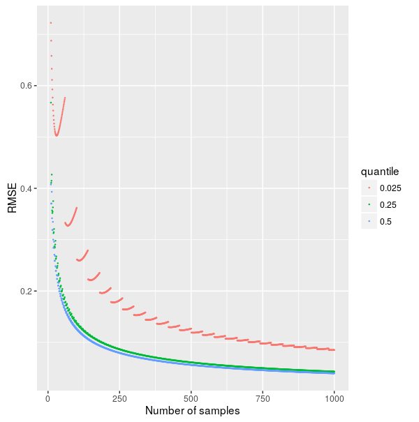
And here is the result:
Accuracy depending on method
The method we used above to estimate the population quantile based on sample’s ordered statistics is not the only one. There is a class of quantile estimators based on various weighted sums of order statistics.
As these estimators are already implemented
in R’s quantile function as different “types”, we’ll
save some time and compare them by simulation instead of computing the
integrals.
simulationRmse <- function(p, n, method) {
replicate(10, {
qs <- replicate(300, quantile(rnorm(n), p, type = method, names = F))
sqrt(mean((qs-qnorm(p))^2))})
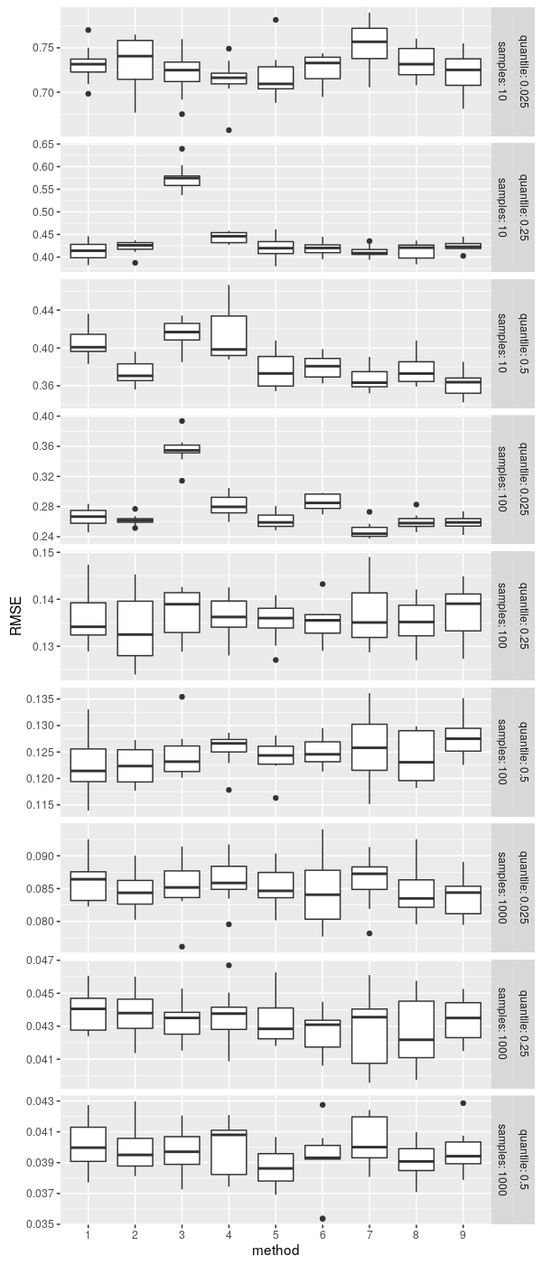
}Since RMSE is now a random quantity, we estimate it 10 times and display as a boxplot to visualize the uncertainty.
Conclusions
- The estimates of more extreme quantiles (such as \(0.025\)) are less accurate. See also Are 50% confidence intervals more robustly estimated than 95% confidence intervals?
- The naive quantile estimator (type 3) is not great on smaller sample sizes; there are many better alternatives. R’s default type 7 fares well.
- Increasing the number of samples improves accuracy (albeit with diminishing returns) and can compensate for an extreme quantile.
- For a parameter that is approximately normally distributed with standard deviation \(\sigma\), to estimate its \(0.025\) quantile within \(0.1\sigma\), we need about \(750\) samples. For the \(0.25\) quantile we need only \(200\) samples.
This article was inspired by an exercise from Bayesian Data Analysis (exercise 1, chapter 10).