Predicting a coin toss

I flip a coin and it comes up heads. What is the probability it will come up heads the next time I flip it?

“Fifty percent,” you say. “The coin tosses are independent events; the coin doesn’t have a memory.”

Now I flip a coin ten times, and ten times in a row it comes up heads. Same question: what is the probability it will come up heads the next time?

You pause for a second, if only because you are not used to seeing a coin land heads ten times in a row.

But, after some hesitation, you convince yourself that this is no different from the first experiment. The coin still has got no memory, and the chances are still 50-50.

Or you become suspicious that something is not right with the coin. Maybe it is biased, or maybe it has two heads and no tails. In that case, your answer may be something like 95% for heads, where the remaining 5% account for the chance that the coin is only somewhat biased and tails are still possible.

This sounds paradoxical: coin tosses are independent, yet the past outcomes influence the probability of the future ones. We can explain this by switching from frequentist to Bayesian statistics. Bayesian statistics lets us model the coin bias (the probability of getting a single outcome of heads) itself as a random variable, which we shall call \(\theta\). It is random simply because we don’t know its true value, and not because it varies from one experiment to another. Consequently, we will update its probability distribution after every experiment because we gain more information, not because it affects the coin itself.

Let \(X_i\in\{H,T\}\) be the outcome of \(i\)th toss. If we know \(\theta\), we automatically know the distribution of \(X_i\):

\[p(X_i=H|\theta)=\theta.\]

As before, the coin has no memory, so for any given \(\theta\), the tosses are independent: \(p(X_i \wedge X_j|\theta)=p(X_i|\theta)p(X_j|\theta)\). But they are independent only when conditioned on \(\theta\), and that resolves the paradox. If we don’t assume that we know \(\theta\), then \(X\)s are dependent, because the earlier observations affect what we know about \(\theta\), and \(\theta\) affects the probability of the future observations.

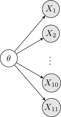
A model with conditionally independent variables is called a Bayesian network or probabilistic graphical model, and it can be represented by a directed graph as shown on the right. The arrows point from causes to effects, and the absence of an edge indicates conditional independence.

Based on our evidence of 10 heads in a row, Bayes’ theorem lets us estimate the distribution of \(\theta\). All we need is a prior distribution – what did we think about the coin before we tossed it?

For coin tossing and other binary problems, it is customary to take the Beta distribution as the prior distribution, as it makes the calculations very easy. Often such choice is justified, but in our case it would be a terrible one. Almost all coins we encounter in our lives are fair. To make the beta distribution centered at \(\theta=0.5\) and low variance, we would need to set its parameters, \(\alpha\) and \(\beta\), to large equal numbers. The resulting distribution would assign non-trivial probability only to low deviations from \(\theta=0.5\), and the distribution would be barely affected by our striking evidence.

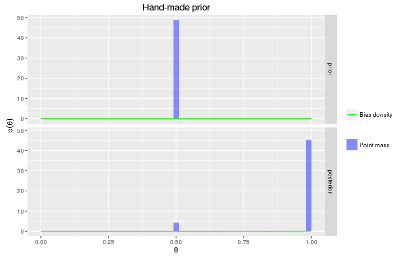
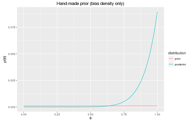
Instead, let’s engineer our prior distribution from scratch. Double-sided coins may be rare in everyday life, but they are easy to buy on eBay. When someone approaches us out of the blue and starts flipping coins, there’s a fair chance they’ve got one of those. Still, we believe in humanity, so let’s assign a point probability of just \(1\%\) to \(\theta=0\) and \(\theta=1\). What about biased coins, such as coins with \(\theta=0.83\)? Turns out they are unlikely to exist. Nevertheless, the Bayesian statistics teaches to be reluctant to assign zero probabilities to events, since then no amount of evidence can prove us wrong. So let’s take \(0.1\%\) and spread it uniformly across the interval \([0;1]\). The remaining \(97.9\%\) will be the probability of a fair coin.

Formally, our prior distribution over \(\theta\) can be specified by its probability density as

\[ p(\theta)=0.979\delta(\theta-0.5)+0.01\delta(\theta)+0.01\delta(\theta-1)+0.001, \]

where \(\delta\) is the Dirac delta function used to specify point probabilities.

Let \(D\) refer to the event that \(X_i=H\), \(i=1,2,\ldots,10\). Then \(p(D|\theta)=\theta^{10}\). By Bayes’ theorem,

\[ p(\theta|D)=\frac{p(D|\theta)p(\theta)}{\int_0^1 p(D|\theta)p(\theta)d\theta} = \frac{\theta^{10}p(\theta)}{\int_0^1 \theta^{10}p(\theta)d\theta}. \]

Now we need to do a bit of calculation by hand:

\[ \begin{multline} \int_0^1 \theta^{10}p(\theta)d\theta=0.979\cdot0.5^{10}+0.01\cdot 1^{10}+0.01 \cdot 0^{10} + 0.001\int_0^1 \theta^{10}d\theta \\ = 9.56\cdot 10^{-4} + 0.01 + 9.09\cdot 10^{-5}=0.0110; \end{multline} \] \[ p(\theta|D)=0.087\delta(\theta-0.5)+0.905\delta(\theta-1)+0.091\theta^{10}. \]

Thus, we are \(90.5\%\) sure that the coin is double-headed, but we also allow \(8.7\%\) for pure coincidence and \(0.8\%\) for a biased coin.

Now back to our question: how likely is it that the next toss will produce heads?

\[ \begin{multline} p(X_{11}=H|D) = \int_0^1 p(X_{11}=H|D,\theta)p(\theta|D)d\theta = \int_0^1 \theta \, p(\theta|D)d\theta \\ = 0.087\cdot 0.5+0.905\cdot 1+0.091\cdot \int_0^1\theta^{11}d\theta = 0.956. \end{multline} \]

Very likely indeed. Notice, by the way, how we used the conditional independence above to replace \(p(X_{11}=H|D,\theta)\) with \(p(X_{11}=H|\theta)=\theta\).

Bayesian statistics is a powerful tool, but the prior matters. Before you reach for the conjugate prior, consider whether it actually represents your beliefs.

A couple of exercises:

1. How does our prior distribution change after a single coin toss (either heads or tails)?
2. How does our prior distribution change after ten heads and one tails?