rank vs. order in R

Published on March 19, 2016; updated on October 30, 2017

A lot of people (myself included) get confused when they are first confronted with rank and order functions in R. Not only do the descriptions of these functions sound related (they both have to do with how a vector’s elements are arranged when the vector is sorted), but their return values may seem identical at first.

Here’s how my first encounter with these two functions went. The easiest thing is to see how they work on already sorted vectors:

> rank(1:3)
[1] 1 2 3
> order(1:3)
[1] 1 2 3

Fair enough. Now let’s try a reversed sorted vector.

> rank(rev(1:3))
[1] 3 2 1
> order(rev(1:3))
[1] 3 2 1

Uhm, ok. I guess I should try to shuffle the elements.

> rank(c(1,3,2))
[1] 1 3 2
> order(c(1,3,2))
[1] 1 3 2

Perhaps 3 elements is too few.

> rank(c(1,3,2,4))
[1] 1 3 2 4
> order(c(1,3,2,4))
[1] 1 3 2 4

Or maybe I shouldn’t use small consequtive numbers?

> rank(c(10,30,20,40))
[1] 1 3 2 4
> order(c(10,30,20,40))
[1] 1 3 2 4

So, where is the difference, and why is it so hard to find?

Definitions

Let’s say we have a sequence of numbers \(a_1, a_2, \ldots, a_n\). For simplicity, assume that all numbers are distinct.

Sorting this sequence yields a permutation \(a_{s_1},a_{s_2},\ldots,a_{s_n}\), where \(s_1\) is the index of the smallest \(a_i\), \(s_2\) is the index of the second smallest one, and so on, up to \(s_n\), the index of the greatest \(a_i\).

The sequence \(s_1,s_2,\ldots,s_n\) is what the order function returns. If a is a vector, a[order(a)] is the same vector but sorted in the ascending order.

Now, the rank of an element is its position in the sorted vector. The rank function returns a vector \(t_1,\ldots,t_n\), where \(t_i\) is the position of \(a_i\) within \(a_{s_1},\ldots,a_{s_n}\).

It is hard to tell in general where \(a_i\) will occur among \(a_{s_1},\ldots,a_{s_n}\); but we know exactly where \(a_{s_k}\) occurs: on the \(k\)th position! Thus, \(t_{s_k}=k\).

Inverse and involutive permutations

Considered as functions (permutations), \(s\) and \(t\) are inverse (\(s\circ t = t\circ s = id\)). Or, expressed in R:

> all((rank(a))[order(a)] == 1:length(a))
[1] TRUE
> all((order(a))[rank(a)] == 1:length(a))
[1] TRUE

In the beginning, we saw several examples of \(s\) and \(t\) being the same, i.e. \(s\circ s = id\). Such functions are called involutions.

That our examples led to involutive permutations was a coincidence, but not an unlikely one. Indeed, for \(n=2\), all two permutations are involutions: \(1,2\) and \(2,1\). In general, permutations \(1,2,\ldots,n\) and \(n,n-1,\ldots,1\) will be involutions for any \(n\); for \(n=2\) it just happens so that there are no others.

For \(n=3\), we have a total of \(3!=6\) permutations. Two of them, the identical permutation and its opposite, are involutions as discussed above. Out of the remaining 4, half are involutions (\(1,3,2\) and \(2,1,3\)) and the other half are not (\(2,3,1\) and \(3,1,2\)). So, for \(n=3\), the odds are 2 to 1 that order and rank will yield the same result.

Any permutation consists of one or more cycles. The non-involutive \(2,3,1\) and \(3,1,2\) are cycles of their own, while \(1,3,2\) consists of two cycles: \((1)\) of size 1 and \((2\;3)\) of size 2. The sum of cycle sizes, of course, must equal \(n\).

It is not hard to see that a permutation is involutive if and only if all its cycles are of sizes 1 or 2. This explains why involutions are so common for \(n=3\); there’s not much room for longer cycles. For larger \(n\), however, the situation changes, and getting at least one cycle longer than 2 becomes inevitable as \(n\) grows.

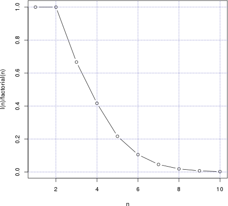
We can easily compute the odds that rank and order coincide for a random permutation of size \(n\). If \(a\) is itself a permutation (e.g. if its generated by sample(n) in R), then \(t=a\). All we need to do is to figure out how many involutions there are among \(n!\) permutations of size \(n\). That number is given by

\[ I(n)=1+\sum_{k=0}^{\lfloor(n-1)/2\rfloor} \frac{1}{(k+1)!} \prod_{i=0}^k \binom{n-2i}{2} \]

(hint: \(k+1\) is the number of cycles of size 2).

I <- function(nn) {
  sapply(nn, function(n) {
    1 + sum(sapply(0:floor((n-1)/2),
      function(k) {
        prod(sapply(0:k, function(i) {
          choose(n-2*i,2)
        })) / factorial(k+1)
      }))
  })
}

n <- 1:10
plot(I(n)/factorial(n) ~ n,type='b')
grid(col=rgb(0.3,0.3,0.7))